Organize data for the multi-state occupancy model fit by occuMS
unmarkedFrameOccuMS.RdOrganizes multi-state occupancy data (currently single-season only)
along with covariates. This S4 class is required by the data argument
of occuMS
unmarkedFrameOccuMS(y, siteCovs=NULL, obsCovs=NULL,
                           numPrimary=1, yearlySiteCovs=NULL)
Arguments
- y
An MxR matrix of multi-state occupancy data for a species, where M is the number of sites and R is the maximum number of observations per site (across all primary and secondary periods, if you have multi-season data). Values in
yshould be integers ranging from 0 (non-detection) to the number of total states - 1. For example, if you have 3 occupancy states,yshould contain only values 0, 1, or 2.- siteCovs
A
data.frameof covariates that vary at the site level. This should have M rows and one column per covariate- obsCovs
Either a named list of
data.frames of covariates that vary within sites, or adata.framewith MxR rows in the ordered by site-observation (if single-season) or site-primary period-observation (if multi-season).- numPrimary
Number of primary time periods (e.g. seasons) for the dynamic or multi-season version of the model. There should be an equal number of secondary periods in each primary period.
- yearlySiteCovs
A data frame with one column per covariate that varies among sites and primary periods (e.g. years). It should have MxT rows where M is the number of sites and T the number of primary periods, ordered by site-primary period. These covariates only used for dynamic (multi-season) models.
Details
unmarkedFrameOccuMS is the S4 class that holds data to be passed
to the occuMS model-fitting function.
Value
an object of class unmarkedFrameOccuMS
See also
Examples
# Fake data
#Parameters
N <- 100; J <- 3; S <- 3
psi <- c(0.5,0.3,0.2)
p11 <- 0.4; p12 <- 0.25; p22 <- 0.3
#Simulate state
z <- sample(0:2, N, replace=TRUE, prob=psi)
#Simulate detection
y <- matrix(0,nrow=N,ncol=J)
for (n in 1:N){
probs <- switch(z[n]+1,
c(0,0,0),
c(1-p11,p11,0),
c(1-p12-p22,p12,p22))
if(z[n]>0){
y[n,] <- sample(0:2, J, replace=TRUE, probs)
}
}
#Covariates
site_covs <- as.data.frame(matrix(rnorm(N*2),ncol=2)) # nrow = # of sites
obs_covs <- as.data.frame(matrix(rnorm(N*J*2),ncol=2)) # nrow = N*J
#Build unmarked frame
umf <- unmarkedFrameOccuMS(y=y,siteCovs=site_covs,obsCovs=obs_covs)
umf # look at data
#> Data frame representation of unmarkedFrame object.
#> y.1 y.2 y.3 V1 V2 V1.1 V1.2 V1.3
#> 1 0 1 2 -0.11960214 0.18685187 -0.5903072 1.3820218 0.03190134
#> 2 0 0 0 -0.80760289 -0.16363905 -1.0025067 -0.9556651 0.49056568
#> 3 0 0 1 0.09131803 -0.08830558 -1.1794174 1.5567544 -0.90426101
#> 4 0 0 0 0.92576093 0.63591746 -1.5027029 -1.5648374 -0.99417265
#> V2.1 V2.2 V2.3
#> 1 -0.4138958 0.1806095 -0.5340386
#> 2 0.0556834 -0.4984706 1.4706609
#> 3 0.2250390 -0.2825336 -0.3444178
#> 4 -0.9267889 1.4876641 -0.2971293
#> [ reached 'max' / getOption("max.print") -- omitted 96 rows ]
summary(umf) # summarize
#> unmarkedFrame Object
#>
#> 100 sites
#> Maximum number of observations per site: 3
#> Mean number of observations per site: 3
#> Number of primary survey periods: 1
#> Number of secondary survey periods: 3
#> Sites with at least one detection: 41
#>
#> Tabulation of y observations:
#> 0 1 2
#> 235 48 17
#>
#> Site-level covariates:
#> V1 V2
#> Min. :-2.22566 Min. :-2.1045
#> 1st Qu.:-0.67515 1st Qu.:-0.4677
#> Median :-0.06307 Median : 0.1904
#> Mean :-0.06273 Mean : 0.1776
#> 3rd Qu.: 0.38793 3rd Qu.: 0.7481
#> Max. : 2.26820 Max. : 2.6442
#>
#> Observation-level covariates:
#> V1 V2
#> Min. :-3.82519 Min. :-2.92663
#> 1st Qu.:-0.81132 1st Qu.:-0.63486
#> Median : 0.01573 Median : 0.05006
#> Mean :-0.02842 Mean :-0.03721
#> 3rd Qu.: 0.70258 3rd Qu.: 0.62629
#> Max. : 3.85176 Max. : 2.58788
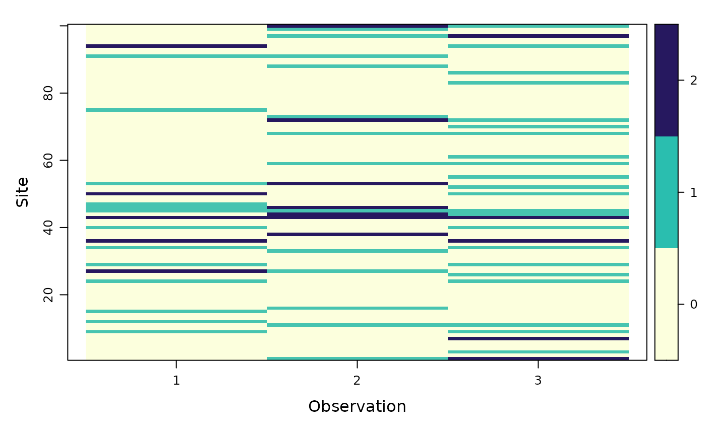
plot(umf) # visualize
 umf@numStates # check number of occupancy states detected
#> [1] 3
umf@numStates # check number of occupancy states detected
#> [1] 3